Part 2-Varying Attributes

    In Part 1 of the Getting Started tutorial you accomplished the following tasks:

1. Used the Block Diagram Editor (BDE) to construct models
2. Generated transactions
3. Defined transaction variables
4. Used queues as part of the system model
5. Created flows
6. Displayed results and analyzed simulation results

    Tutorial Goals

The following is a summary of the concepts and tasks you will learn in Part 2:

1. Define parameters
2. Use parameters in the simulation of the model
3. Save the results to view after the simulation has completed

    Block Diagram

In this session, you will extend the model developed in Part 1 of the tutorial. Previously, you placed a value of 1.0 for the mean time_distribution parameter in the Traffic block and 2.5 as the upper-bound value for the execution time parameter. This simple method of parameter definition is sufficient for a single run of a simulation, but not sufficient when multiple simulations must be run each with different parameter settings.  What is required is a mechanism to modify all the important parameters of the simulation from a single location. In C++ or SystemC code, you would provide something like the following in the main or top file:

Master = new Master("Processor", 4, 0x4c, false, 300);

The above textual statement represents a single location for the definition of (parameter) values for the instance Master.  VisualSim offers a graphical method to perform the same operation. In this case, one would instantiate two global simulation parameters - the "mean of the input rate" and the "upper-bound of the execution time".

A name and associated value is provided for the two parameters. We will start with the model from Part 1. 

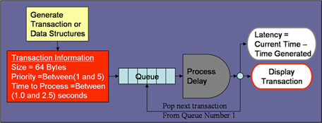
Figure 1: System Block Diagram

The implementation in VisualSim of Figure 1 along with its global parameters is shown in Figure 2.

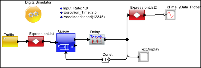
Figure 2: VisualSim model with Parameters

    Now associate the two parameters in Traffic and Expression blocks respectively as shown in Figure 3.

VisualSim Tutorial Model Location

The completed model you are going to build in this tutorial is contained in the following location:

    $VS/VS_AR/doc/Training_Material/Tutorial/WebHelp/Tutorial/Getting_Started/Part2.xml

    Construction Steps

1. Open the block diagram created in Part 1 of this tutorial using menu File > Open File and choose the location where you stored Part1.xml.
2. Drag three instances of Parameter= from ModelSetup > Parameter and place it on the block diagram.
3. Right-click and select Customize Name to enter the name.
4. The first parameter name is Input_Rate, the second parameter is Execution_Time and the third is Modelseed.  
5. Enable Show name to view the entered parameter name after you click submit. 
6. Double-click each parameter and modify its value. 
7. Note: You can also add comments after the value by placing them within /* .... */.
8. Populate the block parameters for the Transaction_Source and the Processing blocks as shown in Figure 3.
9. Save this diagram in the same location as Part1.xml by selecting File > SaveAs with filename Part2.xml.

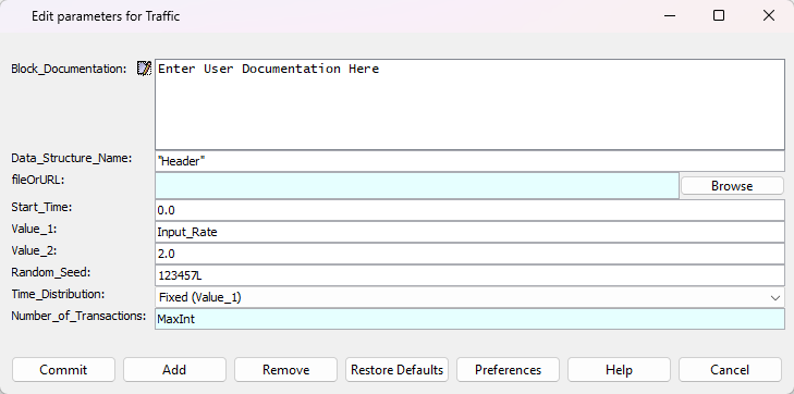
Figure 3-1: Using parameters in the Transaction_Source block

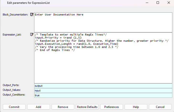
Figure 3-2: Using parameters in the Expression List block

Run the simulation with the different parameters- Run 1, Run 2, and Run 3 and review the results after each simulation run. Run the simulation with the parameters defined in Run 1. After the simulation completes and you review the results, double-click the two parameters, modify  their values for the next run, and re-run the simulation.  Repeat until you have completed the following three Runs.

Run 1: Input_Rate = 1.0 ; Execution_Time = 2.5

Run 2: Input_Rate = 0.8 ; Execution_Time = 2.0

Run 3: Input_Rate = 0.5 ; Execution_Time = 2.5

The Input_Rate is the transaction rate. The upper bound of the Execution_Time is the longest time the system takes to process the transaction.

Also try  additional experiments using other values for the Input_Rate and Execution_Time parameters.

Results

The results from Run 1, Run 2, and Run 3 are shown in Figures 4-1, 4-2, and 4-3, respectively.

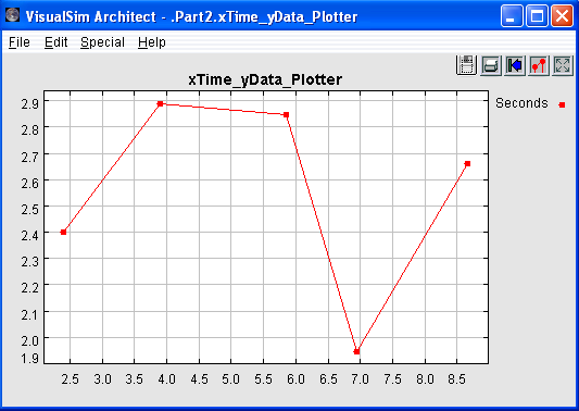
Figure 4-1: Latency plot from Run 1

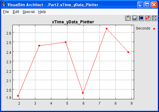
Figure 4-2: Latency plot from Run 2

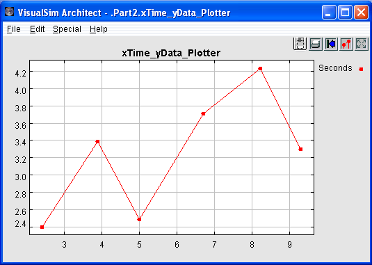
Figure 4-3: Latency plot from Run 3

 Congrats

You have just created the second model in VisualSim!!!

Review this model. Now, we can move to Part 3 of this Lab.