Tutorial Goals
This
tutorial teaches you to use the basic concepts of system modeling
including traffic, behavior, queues, delays and analysis. This
Tutorial also covers the use of the Block Diagram Editor (BDE),
construct
models out of the blocks contained in the VisualSim libraries, run
dynamic simulations, combine different outputs, and interpret the
simulation results.
The following summarizes the concepts and tasks that you learn in this session.
- Understand the Block Diagram Editor
- Generate transactions
- Add content to the transaction
- Manipulate FIFOs/Queues
- Display output and generate latency graphs
Block Diagram Overview
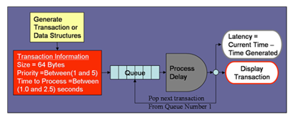
We use the model to study the performance of a system
that has a priority-based FIFO/Queue. The block diagram is shown in
Figure 1.
A traffic generator sends data packets or transactions or data structure to the FIFO. The
FIFO outputs the next transaction after the previous transaction is
processed.

Figure 1: Foundation Example Block Diagram
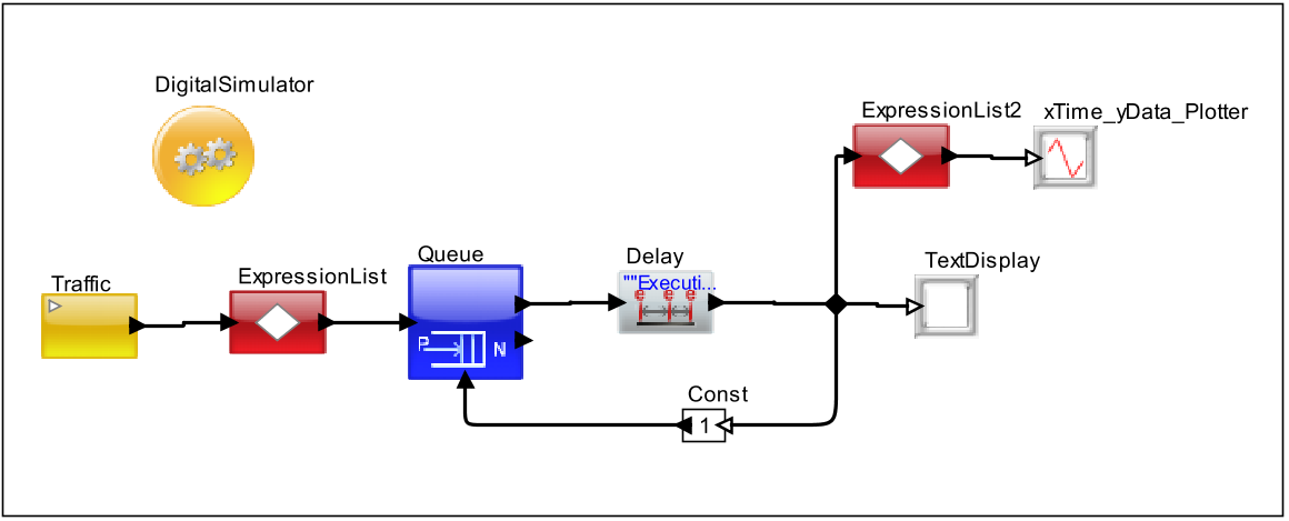
The implementation of Figure 1 in VisualSim is shown in Figure 2.

Figure 2: Foundation Example VisualSim Model
VisualSim Tutorial Model Location
The following location contains the completed model to be built at the end of this tutorial.
- $VS/doc/Training_Material/Tutorial/WebHelp/Tutorial/Getting_Started/Starting_Lab.xml
VisualSim Library Blocks
The following table provides details of the VisualSim library blocks.
S.No.
|
Library Block
|
Description
|
1
|
Digital Simulator
|
The Digital
Simulator implements the discrete-event Model of Computation (MoC). The
simulator maintains a notion of current time, and processes events
chronologically in this time. Used to model elements that change with
time such as hardware, software and networks.
|
2
|
Traffic

|
Outputs a new Data Structure (DS) at time intervals specified by the "Time_Distribution" setting.
A Data Structure is also knowns as a transaction and contains a list of Field Names + Values.
|
3
|
ExpressionList
|
Executes a sequence of expressions in order.
The default block contains one input and one output. The user can add
multiple input and output ports. The graphic shown here is customized
to have two output ports.
|
4
|
Queue
|
Defines multiple
independent parallel queues. Each queue orders the incoming data
structures from highest to the lowest priority.
|
5
|
Const
|
Generates a constant value on the output port every time there is a trigger on the input port.
|
6
|
Text_Display
|
Displays the values arriving on the input port in a text display dialog.
|
7
|
TimeDataPlotter
|
Plots the incoming
data on the Y-Axis against the current simulation time on the X-axis.
Every wire connected to this block input is considered a separate
dataset and plotted separately.
|
Note:
Listen-to-Port feature can be selected by right clicking on any of the
input/output port that you want to debug. After selecting the
Listen-to-Port feature, a blank white window will pop up. Run the model to see the values at the port. For Listen
to Block feature, Right-Click on
the block to debug and select "Kisten to Block". Listen to Block feature cannot be
used for debugging heirarchical blocks as those blocks are used to hold
many different blocks.
Construction Steps
The construction of the model shown in Figure 2 is described below.
- Open a new Model.
- Save this diagram in the desired location by selecting
File->SaveAs and with filename Part1.xml. The .xml extension is
mandatory.
- Define the type of simulation to be performed. As this is a
discrete simulation for performance analysis, add the Digital Simulator.
- Drag the Digital Simulator block from Model Setup->DigitalSimulator.
- Double-click the block and enter the value “10.0” for stopTime.
- Use the default settings for the other parameters.
- Drag and drop the blocks listed below and place them in the BDE as shown previously in Figure 2.
- Traffic->Traffic to generate the transactions based on the data structure template.
- Behavior->ExpressionList to define the transaction fields
and to compute the latency. Note that two ExpressionList blocks are
required.
- Resources-> Queues to define the FIFO.
- Traffic->Delay to emulate the time taken to process a task.
- Results->Text_Display to show the contents of the
transaction after coming out of the Queue and finished the processing
delay.
- Results->TimedDataPlotter to display an XY graph of transaction latency vs. simulation time.
- Full_Library --> Math Operations->Math and Trig->Const
to specify the Queue number to pop. Right-click the Const block and
select Appearance -> Flip Ports Horizontally.
- Click but not drag the Relation button in the Menu bar. A black
diamond will be placed in the BDE. This can be used to define a fan-out
connection of the output of the Delay block.
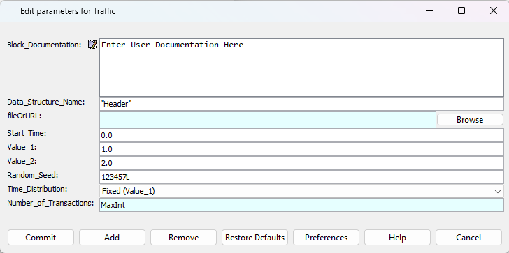
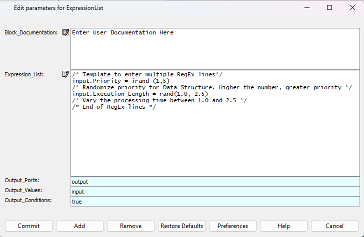
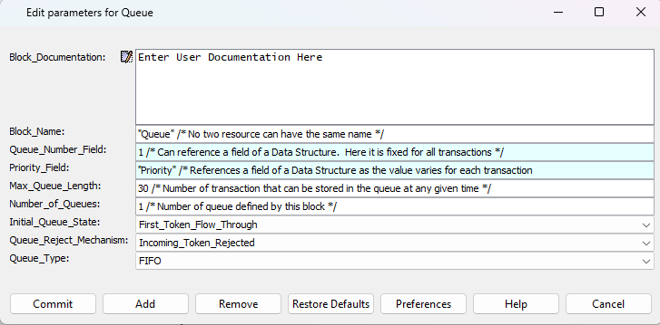
- Populate the block parameters as shown
in Figures 3 to 7. No change is required for the Const,
TimedDataPlotter, and Text_Display blocks. The Data Structure
contains 6 "Header" fields and the field content can be used in the
rest of the model.

Figure 3: Transaction Source
Figure 4: ExpressionList
Note that the purpose of using
expression input.Priority = irand(1,5) is to assign a random value
between 1 and 5 to the Data Structure field Priority. "input"
identifies the data structure and is the name of the block port through
which the data structure enters. If the block has multiple input ports,
then the user must use the name of the respective port to identify the
data structure that will be used in the Expression List block. Two new
fields called Priority
and Execution_Length are added to the Data Structure called input.
The Parameter Output_Ports is a list of all the output ports. The block
can have multiple output ports.The Parameters Output_Values and Output_Conditions must
match the same number of items as Output_Ports. The corresponding value
is sent out on the respective output port.
The parameter Output_Conditions defines whether the data in
Output_Values must be sent out on the port listed in Output_Ports. The
Condition can be true or false, which is evaluated from an Expression.

Figure 5: Queue
Figure 6: Delay
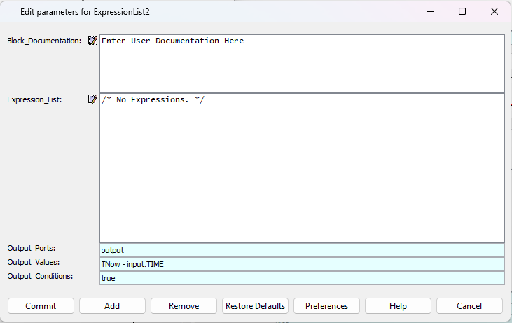
Figure 7: Foundation Example ExpressionList2
Note that the expression TNow - input.TIME returns the end-to-end
latency in the system. TNow is the current simulation time stamp and
input.TIME is the time at which the transaction was generated by the
Traffic block. When a Traffic block generates a data structure, it
places the current time in the TIME field. The Expression_List
parameter does not contain any
expressions. The Output_Values can be an expression containing
equations, transaction if-else, parameters and variables.
- Connect the blocks as shown in Figure 2. There are two different types of connections in the model, one-to-one and one-to-many.
- Port-to-port connections (one-to-one): To connect, click on the
right port of the block, hold down the mouse and drag up to the left
port of the block to be connected or vice versa. This forms a wire
between the source and destination ports. The wire does not add delays
to the transfer; it simply displays the connection between the ports.
It is not sufficient to move one port over the other port. If the
connection is made correctly, the wire is displayed as a thick line. If
the connection is incomplete, the line is thin and disappears when
other actions are performed.
- Many-to-one connections: Use the black diamond or Relation
button. You can place the relation on the BDE by using the control
button + left-mouse click at the location where the Relation must be
placed, or by clicking on the Relation button on the menu. In the
latter case, the relation is placed in the middle of the BDE.
- About Relation: Click the Relation icon and move it to the
appropriate location for aesthetic connectivity. To connect the
relation to the block port, hold down the control button and draw a
line from the relation to the port. If this operation is performed
correctly, the lines are thick. It is not sufficient to simply place
the relation over a wire. All the wires must be connected to this
diamond.
- Block Parameter: Every block contains attributes which can be
defined by the user. The latency calculation in ExpressionList2 has
been entered directly into the Output_Values field and not in the
Expression_List field.
- Block Ports: All blocks have polymorphic ports. This means that
the block determines the right transaction that flows through any port.
There are a few blocks that have preset data types at their ports and
the user the must ensure the right data types is sent to such ports.
The Queue ‘pop’ port requires either an integer or an array.
- Click on the Run button on the VisualSim toolbar to start the simulation.
- The results are displayed both at the text window and the plot (refer to Figures 7 and 8).
Results
Plot of the transaction latency vs. simulation time
Figure 8: Plot of the Transaction Latency vs. Simulation Time
Figure 9: Transaction after the flow has completed
A few things to note.
- The value in the latency field is calculated from the time that
the transaction was generated to the time it completed the processing.
Every transaction is generated with a timestamp field called TIME. TNow
is the current simulation time. Notice that the latency increases
steadily for the first few transactions and then reduces for the fifth
transaction.
- Every transaction has the 6 header fields. A transaction can have
any number of additional fields. Notice that the Execution_Length and the Priority
are different for each transaction. Field ID is a sequence number for
transactions generated by the same source. Notice that these
transactions arrive out-of-order at the destination. This is because
the "Queue" block reorders them in the FIFO, based on priority, before
sending them out.
FAQ
- Why does the latency plot show an increase for the newer transactions?
- Due to queuing of traffic data structures at the "Queue" block,
the latency increases until the output processing can stabilize with
the input rate.
You have just created the first model in VisualSim!!!
Review this model and proceed to Part 2.
Now, we can move to Part 2 of this Lab.
